Wind Loading on a Bridge with SOFiSTiK
Written and presented at the SOFiSTiK Seminar 2016 by:
Prof. Dr.-Ing. Casimir Katz
Supervisory board member, SOFiSTiK AG
Summary
SOFiSTiK has a relatively long history for several aspects of wind analysis in the time domain. The following paper will show the various aspects of a bridge with various possibilities. It is a real bridge in South-East Europe. Still, some parameters have been simplified, and only one construction stage is considered.
1 Location and Wind Parameters
The location is in the mountains, and a considerable turbulences of the wind should be expected. Based on the map of the atmospheric wind conditions, an asymptotic wind speed of 75 m/sec has been selected. The local topography is quite complex. But it has been assured, that based on a roughness value of zo = 1.0 m, a standard wind and turbulence profile could be used and established with SOFiLOAD for the 10 min wind with a return period of 50 years:
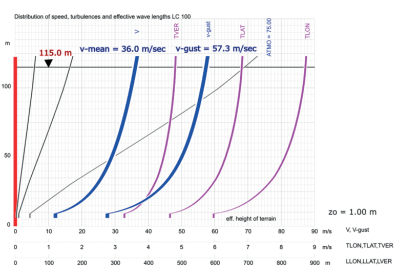
For a construction stage, the local authorities could provide an allowance for a lower value of the return period, and the final stage could be required to be designed with a 120 year return period. The unfavourable wind direction has been chosen to be perpendicular to the bridge.

The longitudinal turbulence intensity at deck height is larger than 24%, the vertical intensity is still larger than 12%. The wind parameters are based on the ESDU 85020 [2] and ESDU 86010 [3] where enhanced formulations of the turbulence and coherence have been developed by various experts in wind engineering including Prof. Alan Davenport. The wind spectrum used is that of Karman which also the base of the Eurocode, but has additional information for the vertical and lateral turbulences.
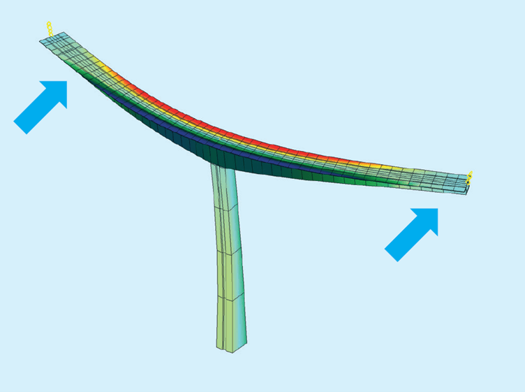
2 System of the Bridge
It is a construction stage of the bridge with a height of 115 m and a full span of 235 m. Two cantilevers expand 120 m to each side with a derrick at the tip.
The height of the sections varies between 4.0 and 13.0 m. The sections of the pier are nearly quadratic but have slightly inclined faces. The logarithmic damping decrement d of the bridge is assumed to be 5 % for the pier and 3 % for the prestressed cantilevers.
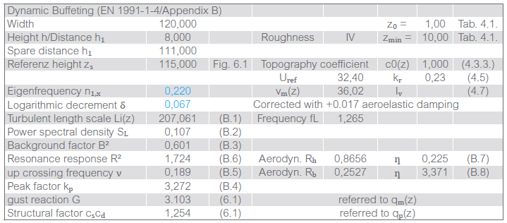
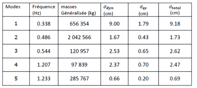
The foundation has been defined with a finite stiffness but without damping. The eigenfrequencies are calculated as follows:
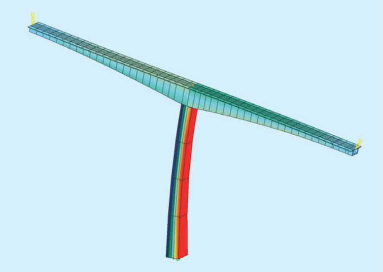
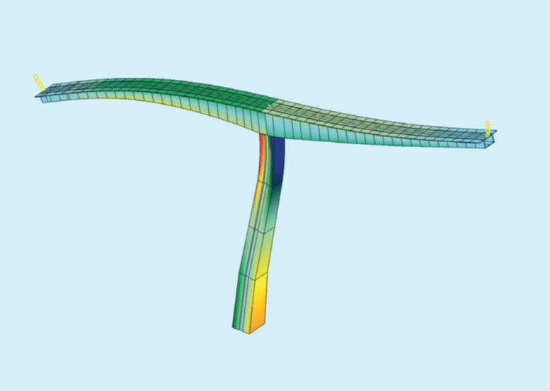
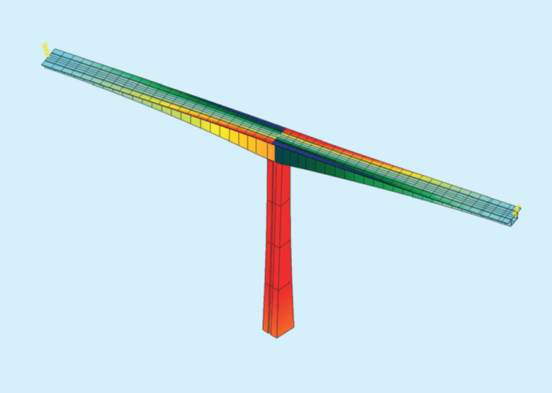
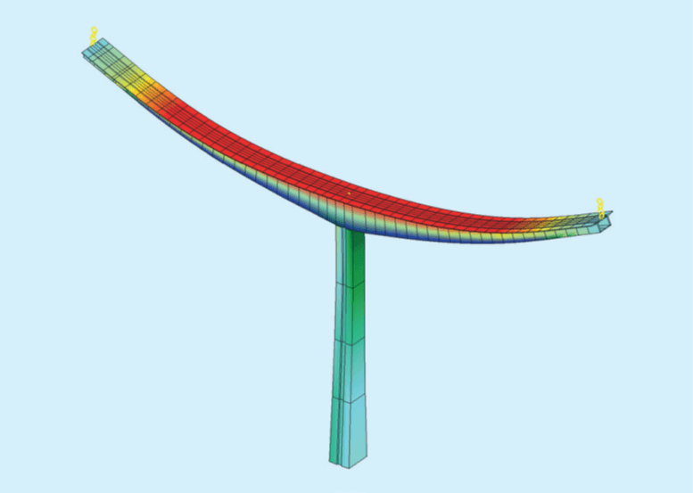
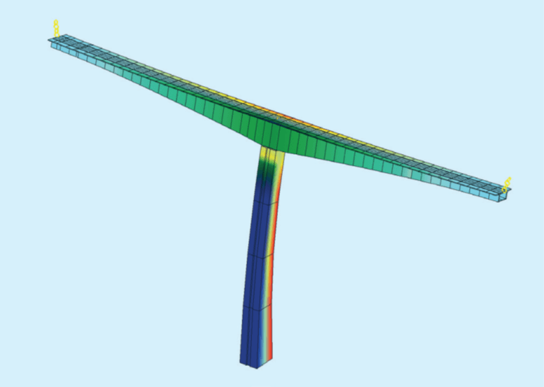
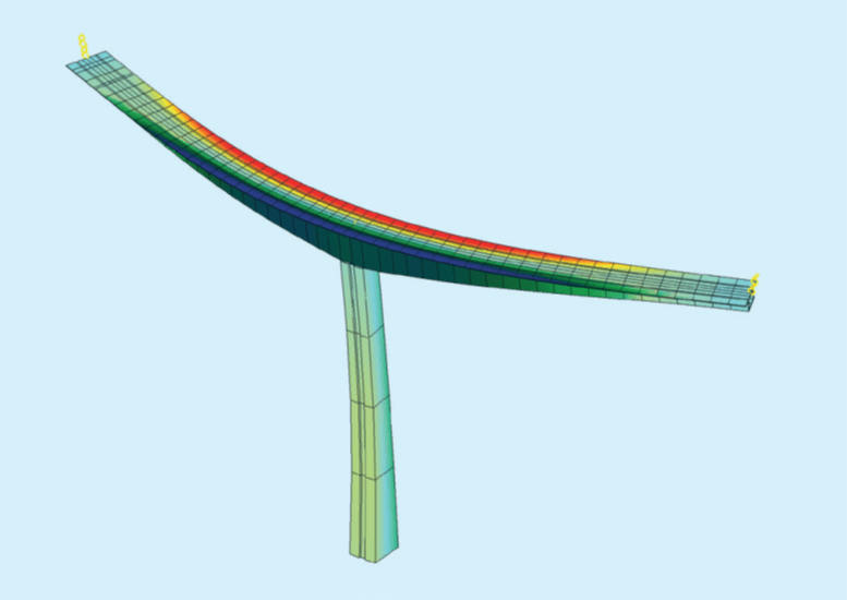
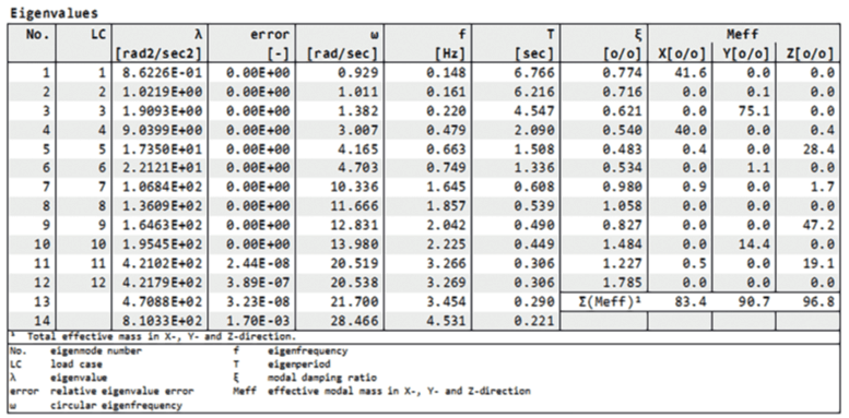
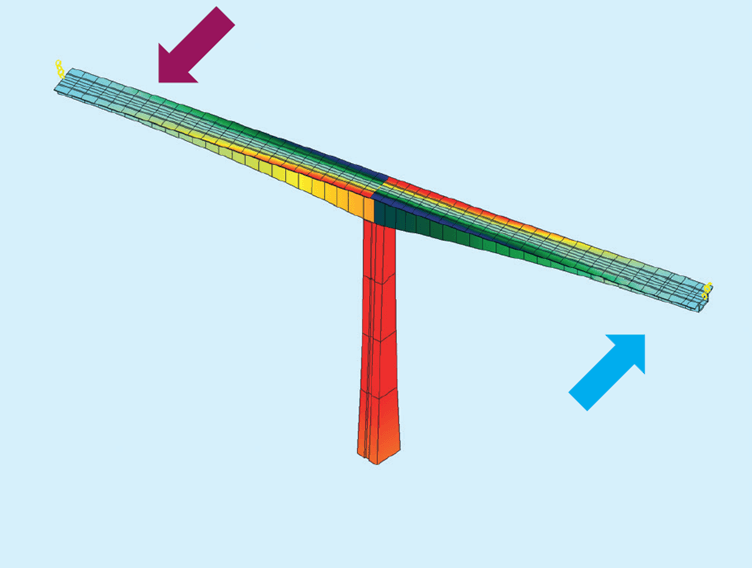
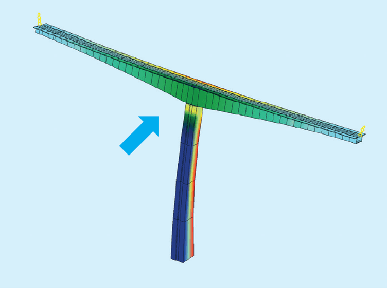
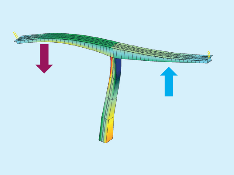
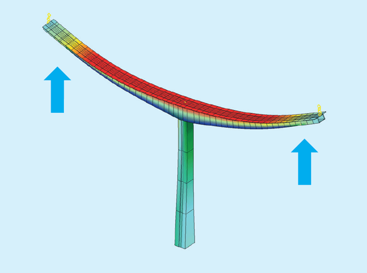
The first is bending mode of the pier along the bridge, the second a torsion of the pier, the 3rd is the bending in the transverse wind direction. The 4th and 5th are vertical bending of the cantilevers, while the 6th is the bending of the cantilever in the transverse direction.
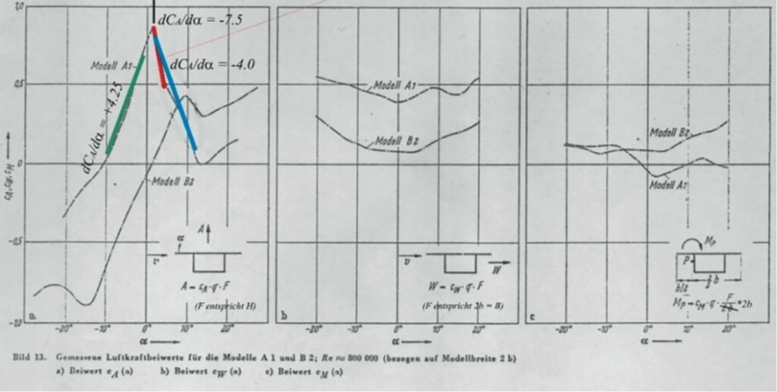
The higher modes are higher bending modes of cantilevers and pier. For the drag coefficients wind tunnel test or CFD analysis have to be considered. But for the section with a smaller height, wind force coefficients have been published. (Kloppel + Thiele: Modellversuche
im Windkanal zur Bemessung von Brucken gegen die Gefahr winderregter Schwingungen. Der Stahlbau, 1967) Selecting Model A1 with a ratio of H/ B=0.3:
It has to be remarked, that the values in the left most diagram from are too high compared to an airfoil, the legend to the paper says that all values are referenced to the full width, but the text makes a reference to the height which seems to be more reasonable.
A special concern is how to treat the wind coefficients with respect to the variant sections. Even if the flow conditions would not change, not all the coefficients depend on the width of the bridge deck, and the drag coefficient should be scaled with the variant height.
But if the drag coefficient is referenced to the height of the section, while the lift coefficient is taken to the width B of the section and the moment is calculated relative to the upper midpoint and referenced to the product B*H, a more uniform distribution could be expected. For an incidence of 0° we then will have the coefficients for model A1: ca=0.26(B), cd = 1.2(H), cm = 0.58 (BH).
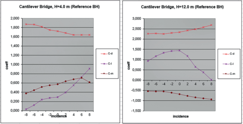
These values are also confirmed by a CFD analysis of the sections. The drag coefficient is referenced to the height of the section, while the lift coefficient is taken to the width B of the section and the moment is calculated relative to the upper midpoint and referenced to the product B*H.
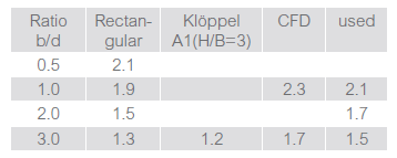
The drag coefficients differ. The values based on the height H for various ratios and different shapes are compared in the following table:
The following pictures show the CFD velocity distribution for different sections and incidences:
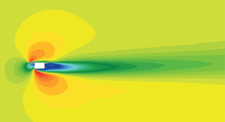
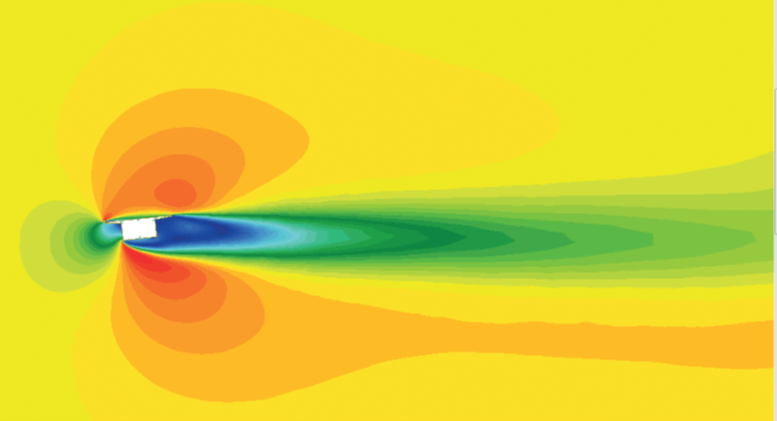
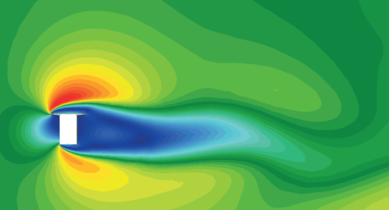
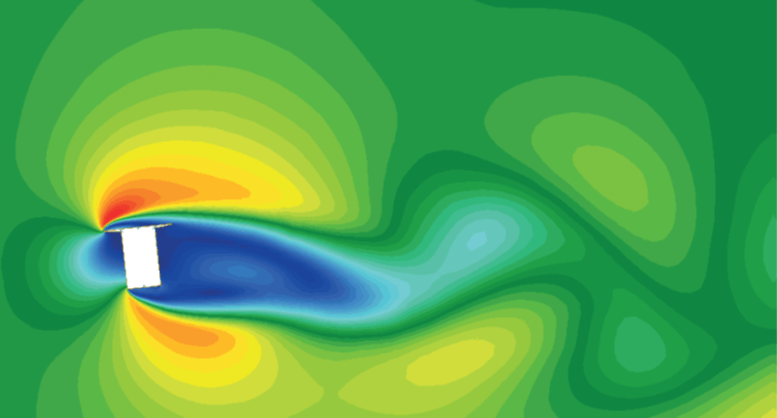
angle of incidence
The CFD analysis uses the full scale and a turbulence intensity of 20 % and inclined representation of the flanges. Thus the results do not match the experiments of the Kloppel A1 wind tunnel. But the sensitivity of the section with respect to negative slopes of the lift and moment coefficients, giving concern to dynamic instabilities (galloping and torsional divergence) can be clearly verified. A special issue is how to interpolate the wind coefficients
along the bridge depending on the height.
For now, the table itself is not interpolated; thus it has to be defined for every individual section, or it should be defined at least based on the BH reference scheme.
In the following analysis, we apply a rather simple scheme based on A1: The drag coefficient is scaled with the height, lift and moment coefficients are taken to be constant. The wind forces on the derricks at the cantilever end will be neglected in this study.
3 Static Analysis
For the static analysis, the gust wind speeds are converted to loads based on the wind coefficients.
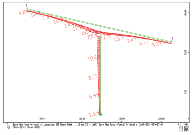
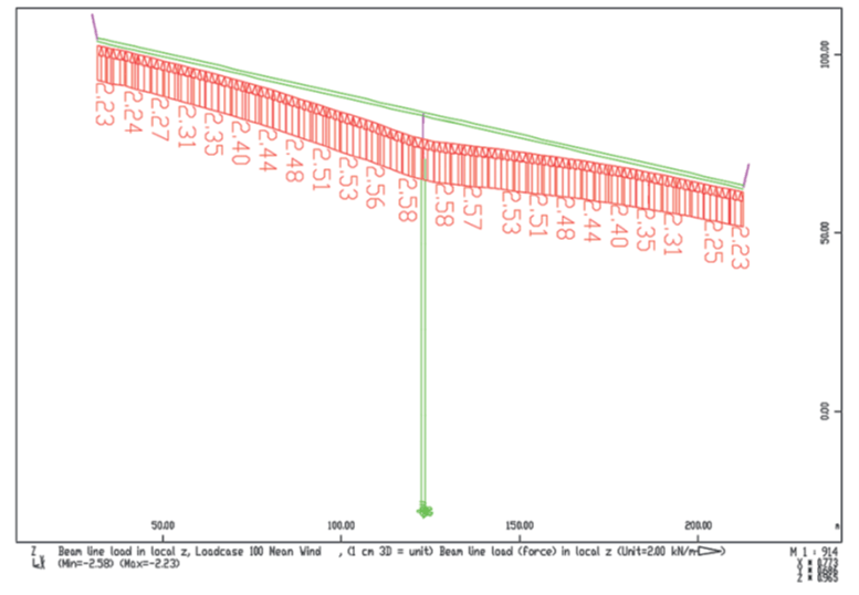
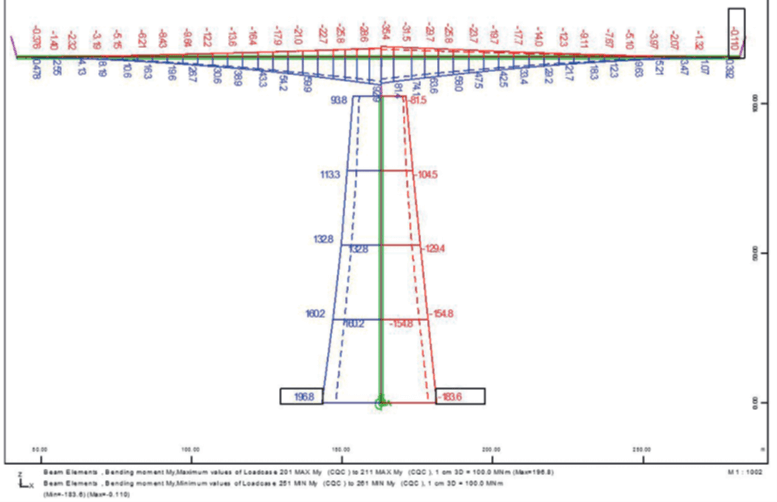
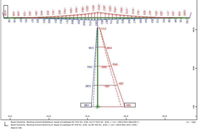
The resulting maximum main bending moment is 432.5 MNm for the bridge. The bending moment in the transverse direction is according linear theory 149.1 MNm for the bridge and 879.5 MNm for the foot of the pier. Second-order effects increase the moment to 915.1
MNm, which is an increase of 3.9 % and allows neglecting 2nd order effects in the dynamic analysis.
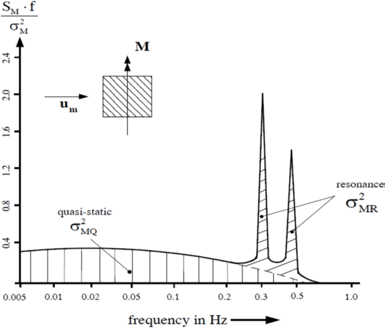
4 Spectral Analysis
The spectral response for a single frequency is defined by a background and a resonance response. To get a correct answer we have to account for the negative aeroelastic damping, evaluated with δ = -0.01 as shown in Figure 4.
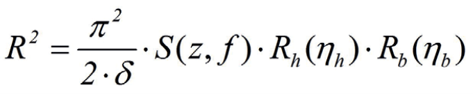
However, this approach does not account for the correct loading of each cantilever, in that case the width should be reduced to 60 m yielding a gust reaction of 3.62.
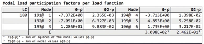
If the combined response for multiple eigenforms is required, the first step is to establish a partial wind load for every eigenform at the most unfavourable location.
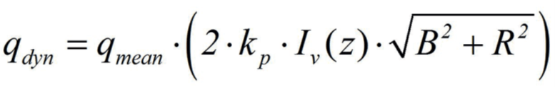
Our approach is to use the same load value based on a pressure of qmean · 2kp · I(z), while the loaded length is based on the coherence.
This is straight forward for any loading in the wind direction only:
dFL=Cd ∙ Aref ∙ qo ∙ 2kp ∙ Ilon
dFV=Cl ∙ Aref ∙ qo ∙ 2kp ∙ Ilon
But if we have vertical movements or turbulences, these will change the angle of attack and we have a second component which is generally larger than the above value obtained by the difference of the lift forces:
dF = 1/2 [Cl (+ ∝dyn ) – Cl (-∝dyn )]∙ Aref ∙ qo ∙ 2kp ∙ Ilon
The range of the dynamic coefficients is influenced by the vertical turbulence intensity and the response factor from the wind spectra, but if we use a linearization with the derivative we get:
dF= dCl/d∝∙ Aref ∙ qo ∙ 2kp ∙ Iver
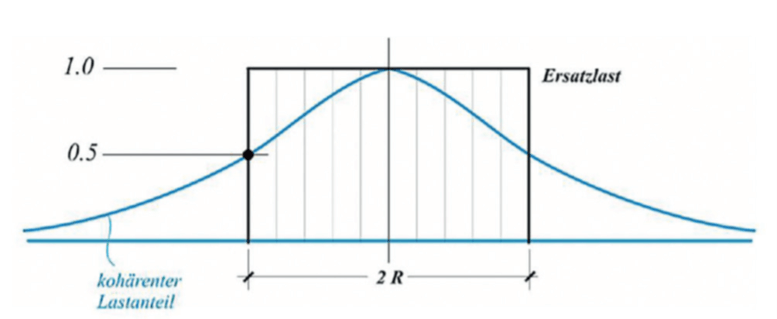
There is no unique way of how to select the equivalent loading. The approach used here is to use a constant loading with the full load along with the double of the half-value distance, another would be to model the distribution with the coherence, another is to use a load on the full length of the bridge with a reduction by a factor accounting for the reduced
length.
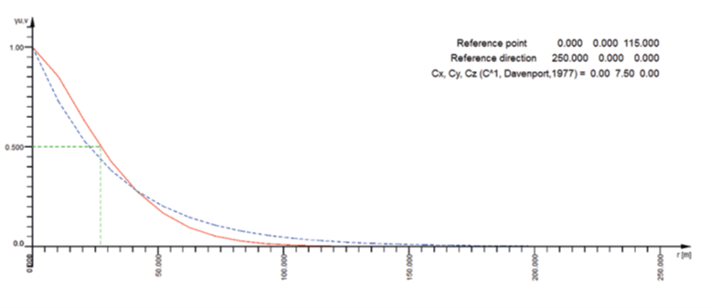
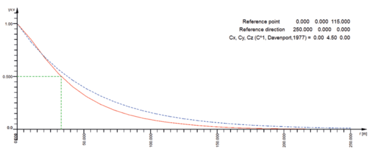
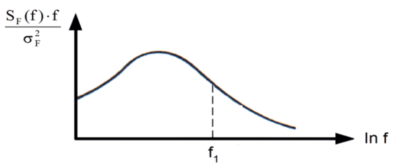
The half-value-distance is obtained by the WTST command in SOFiLOAD:
For every frequency we get the coherence along the bridge at the height of the bridge deck. The red line is the curve according the ESDU, while the blue dashed line is the value obtained with the Davenport formula with Cux = 7.5 and Cvx = 4.5.
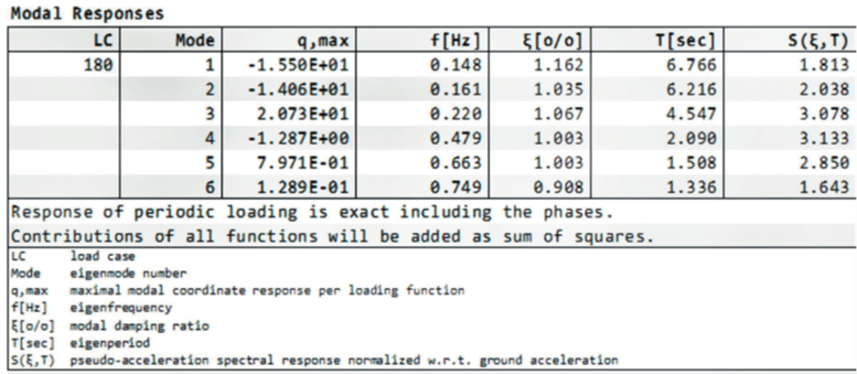
v,v: f = 0.148 Hz, hvd= 33.050 m
u,v: f = 0.161 Hz, hvd= 25.309 m
u,v: f = 0.220 Hz, hvd= 18.612 m
v,v: f = 0.479 Hz, hvd= 12.090 m
v,v: f = 0.663 Hz, hvd= 9.096 m
u,v: f = 0.749 Hz, hvd= 5.468 m
For the load patterns with antisymmetric loading, the peak factor should be adjusted if the length of the cantilevers were not identical and to the probability to have the same unfavourable loading on both sides simultaneously. Then we have to account for the fact, that the values dCL/dα is far away from having a unique value.
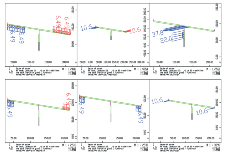
The modal loads are then calculated with different load patterns for every mode (LC item MODB):
Then these modal load cases are combined with the corresponding spectral values. As the coherence is already contained in the load pattern, it is suggested to set the background response to unity.
As stated before, the factor 2kp ・ I(z) has been already included in the definition of the load vector.
The response of all modes is combined by the SRSS/CQC method. It is also possible to specify the modal coordinates explicitly from other sources.
The total response has then to be added to the mean value response. The superposition can use the correct sign for the associated forces if it is done with a factorial equivalent [9]
The background part which can be taken as a quasi-static loading, could be more severe for a different, larger gust size. A rough guide of experience would be to select 50% of the span of a cantilever and 75% of a supported span.
A more detailed elaboration should take 120 m loaded length for the critical gust for the whole bridge, yielding a gust duration of 22 sec. From this a critical gust speed of 49.1 m/s equal to 1.2 ・ qo could be established. For the cantilever alone we have 60 m and a gust duration of 9.5 secs, resulting in a wind speed of 9.5 sec. From this a critical gust speed of 53.4 m/s equal to 2.2 ・ qo could be established.
Although the spectral solution is considerably faster (minutes) in the execution time than the solution in the time domain (hours), it has some important deficits:
• It does not include aeroelastic damping, these values have to be estimated and added to the structural damping beforehand.
• It does not include aeroelastic nonlinearities such as galloping
• It does not allow for structural nonlinearities
• There are considerable simplifications by selecting the load distribution
• The distribution of the forces and moments in the lower eigenforms may ignore important local effects
• In general, the same load distribution should not be used for the background and the resonance response.
Thus there is a lot of expert knowledge required.
5 Transient Analysis
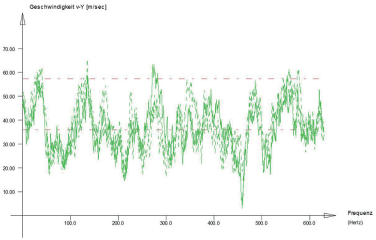
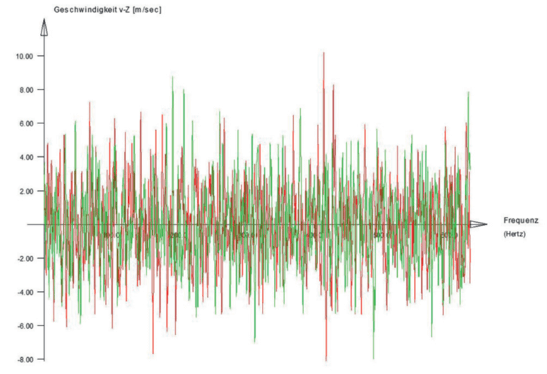
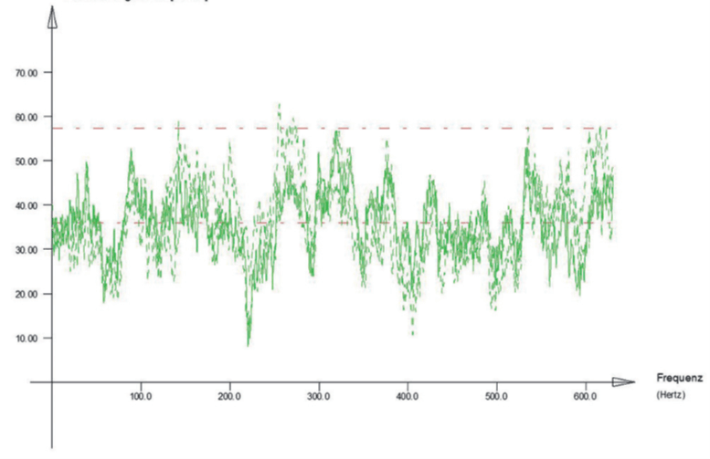
The most general way to account for all nonlinear effects including aeroelastic damping is provided by the possibility to generate artificial time series based on the spectral properties and coherences with SOFiLOAD. Then the structure is interacting in that wind field with a relative wind speed depending on the current angle of attack. This procedure accounts automatically for aeroelastic damping and galloping effects. However, there is a loss of generality and thus, it is required to perform different runs, the next pictures show two different time histories for the two endpoints. Due to the coherence effects, the velocities
are not in phase.
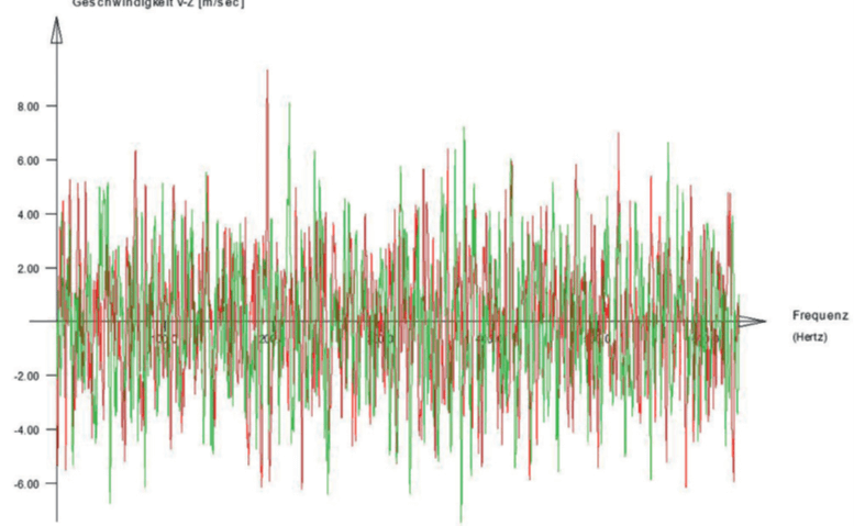
The generated histories depend on the frequency content of the applied spectra. For 10 min wind, the lowest frequency used should be below 0.0017 Hertz. The number of runs required is subject to discussions, but there are some hints in the literature. EN 1998-1 states that for the nonlinear time history analysis of earthquakes at least three runs are required, and the design has to be done for the maximum.
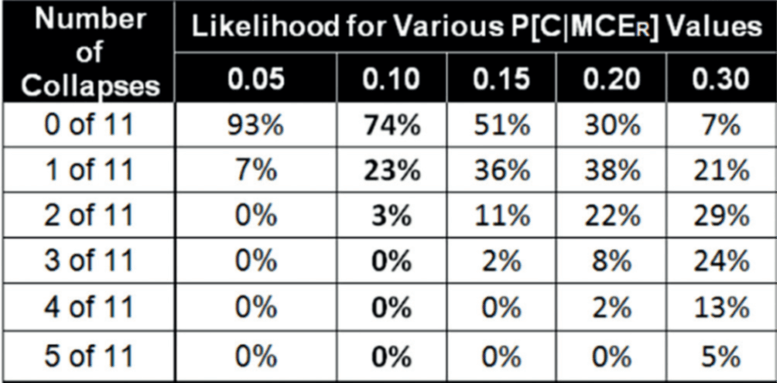
If five or more runs are performed, the mean value can be used. This second provision is difficult if we have a nonlinear analysis with possible failures. Recent research of the ASCE 7-10 Chapter 16 Team has established a better rule. They require to have a minimum of 11 runs. The table specified below shows that for a true collapse probability of 0.10 there is still the chance of 23 % to get one collapse, but very unlikely (3 %) that are two collapses.
From that follows that for risk categories I and II one collapse out of ten is acceptable, but not two. And for risk category III or IV no collapse is allowed out of those eleven cases.
from the time history analysis
Summary
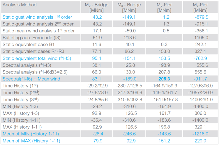
The different approaches yield different results. The above table compares all methods. While the values for the bridge show a good agreement, there are significant deviations for the pier. The lower eigenforms apparently do not allow a precise modelling of the bending behaviour. The ratio of the My-values is about 5 in the first Eigenform, about 3 in the Spectral analysis and about 2 in the final results of the equivalent loadings or the transient analysis.
Literature
[1] Kloppel, Thiele: Modellversuche im Windkanal zur Bemessung von Brucken gegen die Gefahr winderregter Schwingungen. Der Stahlbau, 1967.
[2] ESDU. Characteristics of wind speed in the lower layers of the atmosphere near the ground, Part II: single point data for strong winds (neutral atmosphere). Engineering Science Data Unit 85020, London, 1985.
[3] ESDU. Characteristics of atmospheric turbulence near the ground, Part III: variations in space and time for strong winds (neutral atmosphere). Engineering Science Data Unit 86010, London, 1986.
[4] C. Dyrbye and S.O. Hansen. Wind Loads on Structures. John Wiley and Sons Inc, Chichester, 1997.
[5] I. Kovacs. Synthetic Wind for Investigations in Time-Domain. In Structures Congress XII. American Society of Civil Engineers, 1994.
[6] I. Kovacs, H.P. Andra. Traglastnachweis von Turmbauwerken unter dynamischer Windbelastung. Bautechnik, 11:650–661, 1993.
[7] I. Kovacs, H. Svensson, E. Jordet. Analytical Aerodynamic Investigation of the Cable-Stayed Helgeland Bridge. Journal of Structural Engineering (ASCE), 118:147–168, 1992.
[8] H. Svensson, Cable-Stayed Bridges, Wiley, Berlin, 2012
[9] C. Katz, Anmerkungen zur Uberlagerung von Antwortspektren, DACH Mitteilungsblatt in Bauingenieur 84 Heft 3, 2009
[10] https://commons.wikimedia.org Picture form A. Christaras of Metsovikis Bridge